Quick answer
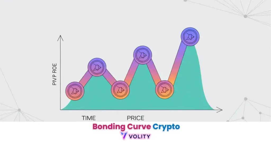
A bonding curve in crypto is a mathematical formula that sets a token’s price based on its supply: as more tokens are bought, the price rises along the curve, and as they are sold, it falls. Bonding curves power automated market makers and token launches, providing instant liquidity without a traditional order book or counterparty.
DeFi mechanisms like bonding curves involve significant technical and financial risk. While they provide instant liquidity, they are highly susceptible to front-running, price manipulation, and protocol-level exploits.
Always verify the underlying smart contract and only commit capital you can afford to lose. Past performance is not indicative of future results.
Capital at risk.
Bonding curves deliver the foundational mathematics required to automate price discovery and liquidity for decentralized assets. These smart contract protocols identify a token’s value through a predetermined function, ensuring that every purchase or sale results in a predictable and transparent price shift. In 2026, the rise of “graduation” protocols has made bonding curves the industry standard for fair-launch tokenomics in a global market that processes trillions in monthly volume.
The evolution of curve models has moved from simple linear growth to complex augmented structures that fund community projects through “exit tributes.” As regulatory frameworks like the EU’s DAC8 mandate greater transparency, the integration of these curves into institutional DeFi collateral systems is accelerating. This guide examines the mechanics of current curve types and the strategic risks involved in 2026 token participation.
While understanding Bonding Curve is important, applying that knowledge is where the real growth happens. Create Your Free Crypto Trading Account to practice with a free demo account and put your strategy to the test.
Quick takeaways
Here is what matters most for this guide.
- Crypto markets trade 24/7 with high volatility and no central authority.
- Liquidity, execution venue, and self-custody choices shape every trade outcome.
- Furthermore, MiCA and FATF rules now reshape EU and global crypto flow.
Therefore, read on for the full breakdown below.
What is a Bonding Curve and how does it automate DeFi liquidity?
A bonding curve is a smart contract-controlled pricing mechanism that links a token’s value directly to its circulating supply via an algorithmic mathematical function. The smart contract acts as a perpetual counterparty, simultaneously buying and selling tokens at prices determined by the curve formula rather than external market makers. This deterministic model reveals that every transaction’s price is verifiable on-chain, eliminating the “hidden depth” problems found in traditional exchanges (Ethereum.org, 2026).
Bonding curves remove the need for order books by replacing the matching engine with a mathematical function. When you purchase tokens, the smart contract automatically creates new supply and adjusts the price upward according to the curve’s formula, higher supply, higher price. When you sell, the contract burns tokens and reduces the price downward. This perpetual counterparty removes friction because there is no need to wait for an external buyer or seller to arrive (Ethereum.org, 2026).
The reserve backing principle ensures that every token minted has a corresponding deposit of base assets, typically ETH, SOL, or USDC, held in the contract. This reserve guarantees that you can always sell your tokens back to the curve at the price determined by the mathematical function, eliminating the counterparty default risk present in traditional exchanges. The Automated Market Maker (AMM) Crypto: Liquidity Without Order Books framework explains how bonding curves represent a precursor to modern AMM architecture.
Ready to Elevate Your Trading?
You have the information. Now, get the platform. Join thousands of successful traders who use Volity for its powerful tools, fast execution, and dedicated support.
Create Your Account in Under 3 MinutesHow does a Bonding Curve “graduate” to a Decentralized Exchange (DEX)?
Token graduation refers to the automated process where a bonding curve migrates its accumulated liquidity to a permanent DEX pool once a specific market capitalization threshold is reached. The launchpad defines a graduation threshold, typically between $69,000 and $75,000 in market cap, at which point the smart contract automatically wraps the curve’s reserve assets and LP tokens into a permanent Uniswap or Raydium pool (Pump.fun Data, 2026). This transition ensures that early adopters transition from the deterministic pricing model to open-market trading with professional liquidity providers.
The graduation process identifies a key innovation in 2026 token launches: “un-ruggable” liquidity. Protocols typically burn the private keys or liquidity provider tokens associated with the migrated pool, making it mathematically impossible for founders to withdraw the liquidity and abandon the project. This burned LP mechanism removes the default risk that plagued earlier launchpad models where founding teams could drain pools immediately after launch. Over 85% of new Solana-based tokens in 2026 utilize a graduation model to ensure day-one liquidity for retail participants (Pump.fun Data, 2026).
Post-graduation pricing becomes more volatile because the DEX environment exposes the token to traditional market dynamics, supply and demand imbalances, arbitrage trading, and bot-driven volatility. The How to Buy New Crypto Before Listing on Major Exchanges guide explains how early-stage bonding curve participation differs from secondary market trading on decentralized exchanges.
What are the different types of Bonding Curve mathematical models?
Bonding curve mathematical models identify the specific price-to-supply relationship, ranging from steady linear growth to aggressive exponential reward structures. Linear curves (P = m*S) deliver constant price increments per unit of supply, making them ideal for projects prioritizing predictable valuation growth and discouraging extreme speculation. Exponential curves (P = S^n) reward early adopters with accelerating price appreciation as supply grows, creating a powerful incentive for first movers but introducing volatility that deters risk-averse participants.
Sigmoid models (S-curves) combine early aggressive growth with a stabilization phase, mimicking the classic adoption curve seen in biological systems and technology rollouts. The curve starts flat (low price for early adopters), accelerates sharply through the middle phase (rewards growing adoption), and plateaus at maturity (stabilizes price for institutional use). Piecewise curves introduce custom functions used by 2026 enterprise protocols to manage complex collateral requirements, for example, enforcing a linear phase for the first 50% of supply and an exponential phase thereafter. The Smart Contracts: The Self-Executing Code Replacing Lawyers & Banks guide establishes how these mathematical functions translate into smart contract logic and Ethereum Developer Documentation: Smart Contract Mechanics provides the technical foundation for implementing these models.
2026 Bonding Curve Performance and Compliance Benchmarks
Bonding curve performance reveals the capital efficiency of automated liquidity and the growing regulatory reporting requirements for decentralized launchpads in 2026.
| Curve Type | Property | Value |
| Linear Curve | Price Growth | Constant (m * S) |
| Exponential Curve | Reward Model | Early Adopter (S^n) |
| Augmented Curve | Revenue Stream | Exit Tribute (Gitcoin, 2026) |
| Launchpad Cap | Migration Threshold | $69,000 – $75,000 (Pump.fun, 2026) |
| EU Compliance | Reporting Rule | DAC8 (Jan 2026) |
Sources: Data sourced from official protocol specifications and 2026 EU regulatory guidelines. Revenue diversion mechanisms verified via Gitcoin: Augmented Bonding Curves for Public Goods.
Turn Knowledge into Profit
You have done the reading, now it is time to act. The best way to learn is by doing. Open a free, no-risk demo account and practice your strategy with virtual funds today.
Open a Free Demo AccountWhat are Augmented Bonding Curves and “Exit Tributes”?
Augmented Bonding Curves (ABC) are specialized smart contracts that divert a portion of every transaction into a community-governed treasury to fund public goods or protocol development. The exit tribute mechanism charges a programmed fee, typically 2%, when holders sell tokens back to the curve, automatically redirecting that revenue to a DAO treasury rather than to the protocol founder. This design removes the conflict of interest that plagues traditional venture-backed token launches, where founding teams profit directly from token sales while contributing nothing to the ecosystem.
The hatch phase provides the initial reserve backing for the curve by collecting capital from early participants who lock funds for a predetermined period. This lock-in requirement demonstrates participant commitment while building the reserve that guarantees token redemptions. DAOs use augmented curves to create sustainable, automated revenue streams without relying on venture capital or token sales to privileged insiders.
Gitcoin demonstrates this utility in practice: a user selling $1,000 worth of governance tokens back to the augmented curve received $980 in base assets while the $20 (2% exit tribute) was automatically sent to the community grant pool for new developers. Past performance is not indicative of future results. This mechanism reveals how What is a DAO (Decentralized Autonomous Organization) in Crypto? structures use bonding curves to align incentives between founders, participants, and communities supporting public infrastructure.
How do I identify and manage the risks of Bonding Curve launches?
Risk management for bonding curves identifies the specific threats posed by automated front-running, “bundling” by developers, and high-impact slippage. Dev bundling represents the primary abuse vector: a creator purchases the entire early supply using multiple wallets to accumulate 80%+ of the tokens before graduation occurs. This concentrated ownership allows the bundler to dump massive positions immediately post-graduation, crashing the price while retail participants hold worthless tokens. On-chain scanners like Etherscan and Solscan reveal bundling by showing whether the initial curve purchases were distributed across many independent wallets or concentrated in a few addresses.
Sniper bots automate front-running by detecting pending buy orders in the mempool and executing trades ahead of human participants. This forces the original buyer to purchase tokens at a higher price than the initial quote, with the bot capturing the difference as profit. Slippage and price impact become severe on bonding curves because every trade directly alters the supply-to-price ratio, a large order consumes significant liquidity and may result in dramatically worse execution than expected.
EU DAC8 regulations implemented in 2026 require bonding curve launchpads to automate transaction data reporting for tax compliance, eliminating the anonymity that characterized earlier “degen” launchpad activity. This regulatory shift forces participants to acknowledge their participation in formal tax records, fundamentally changing the risk calculus for tax-averse participants. The Slippage in Crypto: Master Execution & Protect Profits guide explains execution best practices, while Polaris Finance: pETH Bonding Curve Technical Specifications provides advanced risk management benchmarks.
Key Takeaways
- Bonding curves algorithmically determine token price based on supply, providing deterministic execution without the need for order books.
- The 2026 graduation protocol automatically migrates bonding curve liquidity to permanent DEX pools once a market cap target is reached.
- Exponential bonding curves reward early adopters with accelerating price increases, while Sigmoid models prioritize long-term stabilization.
- Augmented Bonding Curves utilize ‘Exit Tributes’ to create sustainable, automated funding streams for decentralized organizations (DAOs).
- Slippage and price impact are significantly higher on bonding curves for large orders, as every trade directly alters the supply-to-price ratio.
- EU DAC8 regulations implemented in 2026 now require bonding curve launchpads to automate transaction data reporting for tax compliance.
Frequently Asked Questions
This article contains references to bonding curves and Volity, a regulated CFD trading platform. This content is produced for educational purposes only and does not constitute financial advice or a recommendation to buy or sell any financial instrument. Always verify current regulatory status and platform details before using any trading service. Some links in this article may be affiliate links.
[/coi_disclosure]
What our analysts watch: Bonding-curve launches cluster around three failure and success patterns we monitor on the Volity desk. Time-to-graduation (the threshold at which a token migrates from curve to a standard DEX pool), holder distribution at graduation (concentration risk for the post-graduation chart), and the developer wallet behavior post-graduation (sell pressure). When concentration sits above 50% in the top ten holders, post-graduation charts almost always retrace into the launch range.
Volity operates a trading platform and also publishes educational and analytical content about trading. The content on this page is for educational purposes only and should not be considered financial advice. Volity may benefit commercially when readers open trading accounts through links on this site.
Our content is produced and reviewed under documented editorial standards; comparison and review methodology is published here.